
In April, we published an article showing that Machine Learning (ML) can improve the prediction accuracy of the Cure Rate (CR) in Loss Given Default (LGD) models. This is the second part of our two-part series blog. We test several ML methods on a dataset in the context of LGD Modelling and evaluate the potential of ML techniques within credit risk modelling. Last time, we have seen that the Random Forest (RF) method and the XGBoost technique perform better than the industry standard: Logistic Regression (LR). Next to that, the use of a Neural Network shows great potential. For more background on these techniques, take a look at the first article.
In this second article, we experiment and investigate further potential of ML techniques outside the traditional LGD framework. Usually, a LGD model is split into submodels which are in line with regulatory requirements. This split makes sense in terms of economic interpretation, but we investigate if this also makes sense in terms of model performance. With ML techniques, we do not adhere to the European Banking Authority (EBA) guidelines as we model the LGD directly (without using submodels). To investigate this, we developed this use case together with the Retail Bank Portfolio Management team of NIBC. We use a simulated dataset based on characteristics of the NIBC retail mortgages portfolio. Our use case shows that modelling LGD directly and combining this with ML methods can result in a substantial increase in terms of the prediction performance of a LGD model.
Both econometric modelling and ML techniques are based on statistics. However, the largest difference between the two is that an econometric model is built around several assumptions that simplify the problem. These assumptions work, most of the time, quite well and ensure that the model is understandable and interpretable. A ML model, on the other hand, has less strict assumptions and therefore has more flexibility. This flexibility allows the model to find more complex and non-linear relations, which can improve the prediction performance considerably. This advantage also comes at a cost: as the model becomes more complex, it becomes more difficult to interpret, understand, and validate the working of the model.
Table of Contents
1. Modelling LGD
2. Machine Learning Methods
3. Does Modelling LGD without Submodels Improve the Prediction Performance?
Modeling
For LGD modelling, the EBA sets clear guidelines for risk differentiation and model components to be used. A LGD model is split in two components: a Cure Rate (CR) model and a Loss Given Loss (LGL) model. Using these components, the LGD is calculated as follows:
LGD = CR * LGC + (1 – CR) * LGL
Here, the LGC is the Loss Given Cure, which is the loss given that a client goes back to performing again. In our models, the LGC is assumed to be a fixed percentage of 5%. This split in different components ensures understandable models and makes sense in terms of business interpretation. These EBA guidelines can also be seen as assumptions (or, in this case, restrictions) that simplify the problem, just like econometrics versus ML. However, it is interesting to look at this model’s assumptions from a performance perspective. Is this split necessary and does it improve the performance of the LGD model? The alternative approach is to loosen these restrictions, and model LGD directly (without submodels). We used two types of models: supervised and unsupervised ML techniques.
Machine Learning Methods
To start with the supervised ML techniques, two methods are applied: a Random Forest and XGBoost. These methods are described in the previous blogpost. There, the cure rate was used as the target variable. The target variable in this setup is the realised LGD.
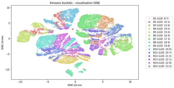
Moving on to the unsupervised ML techniques. This technique is used to discover hidden patterns in unlabelled datasets. The method that is used is a clustering analysis named Kmeans, which involves the grouping of data points. Based on risk drivers, patterns can be discovered of data points behaving in a similar way. For example, a group of clients living in the same area and showing similar payment patterns over time. The algorithm minimises the with-in group distance of each cluster. Using t-distributed Stochastic Neighbor Embedding (tSNE), the groups of clients are visualised in the figure below. In this example, the clients are grouped into 15 categories. We see that the clients representing the clusters lie close to each other. This makes the method quite intuitive.
The clusters do not necessarily focus on the same client characteristics. This is visualised in Figure 2, where we look at four clusters. The figure shows the impact of each risk driver on the four clusters. Clearly, the clients representing the clusters and the corresponding levels of LGD differ substantially. This allows the user to easily zoom into the clusters separately and helps to understand why the clients in the clusters are similar.
Does Modelling LGD without Submodels Improve the Prediction Performance?
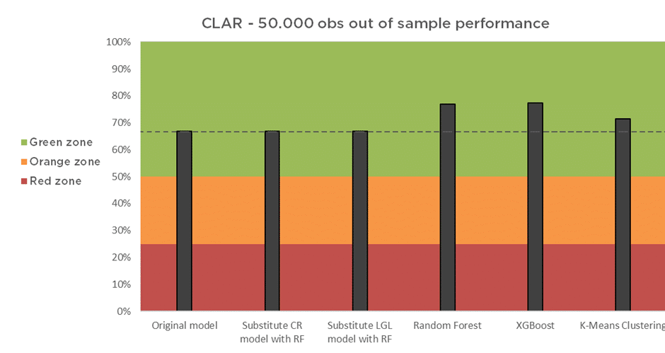
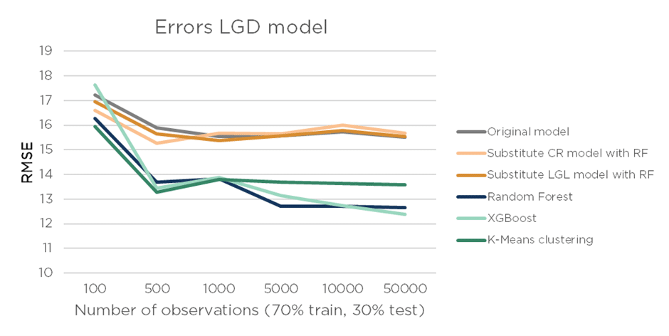
In the two Figures below, we compare six methods of LGD modelling using two performance metrics, CLAR (Figure 3) and RMSE (Figure 4):
- Original model, where CR is modelled with a Logistic Regression and LGL with a Linear Regression;
- Substitute CR model with Random Forest, which is the original model where CR is modelled with a Random Forest;
- Substitute LGL model with Random Forest, which is the original model where LGL is modelled with a RF;
- Random Forest, where the LGD formula is not used but LGD is modelled directly;
- XGBoost, where the LGD formula is not used but LGD is modelled directly;
- K-means clustering, where the LGD formula is not used but LGD is modelled with unsupervised clustering.
As can be seen from Figure 3, all the model combinations have good model performance. Comparing the original model with the two models where we substituted the CR and LGL with a RF, we do not observe much of a difference. However, when we loosen the restriction of the LGD framework (see Equation 1), and we thus predict the LGD directly, we observe a notable increase in the CLAR. Especially the RF and XGBoost methods perform considerably well, which shows that loosening the LGD constraints in combination with using a ML method can substantially increase the performance of a LGD model.
Next to that, in Figure 4, we investigate how the model’s performance evolves when the training dataset becomes larger. More data equals more information, so overall you would expect the models to benefit from having more information to learn form. With only 100 observations, the errors of the different methods are quite comparable. However, as we increase the number of observations, the RF and XGBoost significantly outperform the other methods. So, the ML methods that did not use the LGD formula benefit more from an increase in the number of observations, which is similar to the results found in the previous blogpost.
Concluding, substituting either the LGL or CR model with a Random Forest model (instead of a traditional regression) does not add substantially to the performance of the final LGD model, where the two separate models are aggregated. This limited performance improvement always must be measured against the disadvantages, for example the complexity and interpretability of ML methods.
When we let go of the split in the LGD framework we do see improved performance in terms of CLAR and RMSE. Especially, with a larger number of observations the performance improves substantially. Of course, the LGD model without submodels is currently not allowed given the regulation and this is also not expected to change soon (given the clear interpretation in line with client processes). However, these models could very well serve as a challenger model to compare risk drivers and performance, or they can be used in validation of credit risk models.
What’s next?
Are you interested in how ML techniques would perform on your data? We are happy to help you get the most out of your data using innovative techniques. Please contact Scott Bush at sbush@adc-consulting.com or check our contactpage.
What stage is your organisation in on its data-driven journey?
Discover your data maturity stage. Take our Data Maturity Assessment to find out and gain valuable insights into your organisation’s data practices.